Introduction
Python has become the go-to language for scientific computing and data visualization, and cartography is no exception. With libraries like Cartopy, Matplotlib, and GeoPandas, you can create publication-quality azimuthal equidistant maps with just a few lines of code.
In this tutorial, you'll learn how to:
- Set up a Python environment for cartography
- Create azimuthal equidistant projections centered on any location
- Add coastlines, countries, and custom features
- Draw distance rings and azimuth labels
- Export high-resolution maps for print or web
- Automate map generation for multiple locations
Prerequisites
You'll need:
- Python 3.8 or higher
- Basic familiarity with Python and NumPy
- Understanding of geographic coordinates
Setting Up Your Environment
Installing Required Libraries
Create a virtual environment and install the dependencies:
# Create virtual environment
python -m venv cartopy-env

# Activate it
# Windows:
cartopy-env\Scripts\activate
# macOS/Linux:
source cartopy-env/bin/activate

# Install libraries
pip install cartopy matplotlib numpy shapely geopandas
Note: Cartopy requires GEOS and PROJ libraries. On some systems:
# Ubuntu/Debian
sudo apt-get install libgeos-dev libproj-dev

# macOS with Homebrew
brew install geos proj

# Windows - use conda instead:
conda install -c conda-forge cartopy
Verify Installation
import cartopy
import matplotlib.pyplot as plt
print(f"Cartopy version: {cartopy.__version__}")
print("Setup successful!")
Understanding Cartopy Projections
Cartopy wraps the PROJ library and provides Pythonic access to map projections. The azimuthal equidistant projection is accessed via:
import cartopy.crs as ccrs

# Create projection centered on a point
projection = ccrs.AzimuthalEquidistant(
    central_longitude=-74.006,  # New York longitude
    central_latitude=40.7128    # New York latitude
)
The key parameters:
| Parameter | Description | Default |
|---|---|---|
central_longitude |
Center point longitude | 0.0 |
central_latitude |
Center point latitude | 0.0 |
false_easting |
X offset in meters | 0.0 |
false_northing |
Y offset in meters | 0.0 |
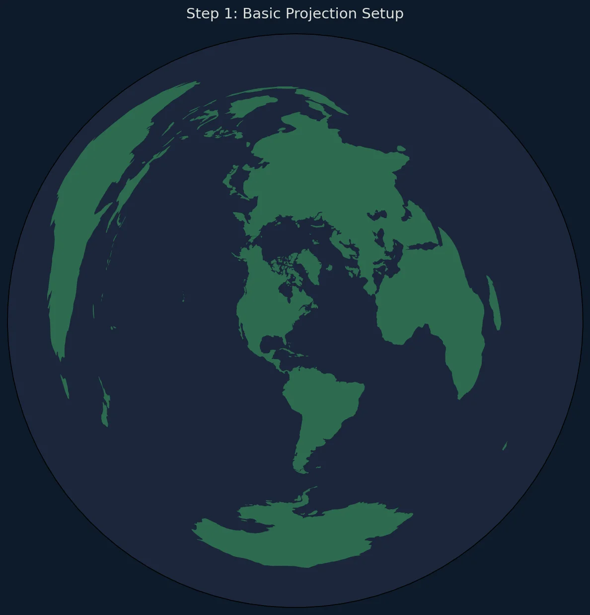
Creating Your First Map
Basic World Map
import matplotlib.pyplot as plt
import matplotlib.path as mpath
import cartopy.crs as ccrs
import cartopy.feature as cfeature
import numpy as np
# Configuration
center_lat = 40.7128 # New York City
center_lon = -74.0060
def set_circular_boundary(ax):
"""Set a circular boundary for azimuthal projections."""
theta = np.linspace(0, 2 * np.pi, 100)
center, radius = [0.5, 0.5], 0.5
verts = np.vstack([np.sin(theta), np.cos(theta)]).T
circle = mpath.Path(verts * radius + center)
ax.set_boundary(circle, transform=ax.transAxes)
# Create figure with dark background
fig = plt.figure(figsize=(10, 10), facecolor='#0d1b2a')
# Create projection centered on our location
proj = ccrs.AzimuthalEquidistant(
central_longitude=center_lon,
central_latitude=center_lat
)
ax = fig.add_subplot(1, 1, 1, projection=proj)
# Use set_global() for full Earth view, then apply circular boundary
ax.set_global()
set_circular_boundary(ax)
ax.set_facecolor('#0d1b2a')
# Add features with proper z-ordering
ax.add_feature(cfeature.OCEAN, facecolor='#1b263b', zorder=1)
ax.add_feature(cfeature.LAND, facecolor='#2d6a4f', edgecolor='none', zorder=2)
ax.add_feature(cfeature.COASTLINE, linewidth=0.5, edgecolor='#84a98c', zorder=3)
ax.add_feature(cfeature.BORDERS, linewidth=0.3, edgecolor='#778da9', zorder=3)
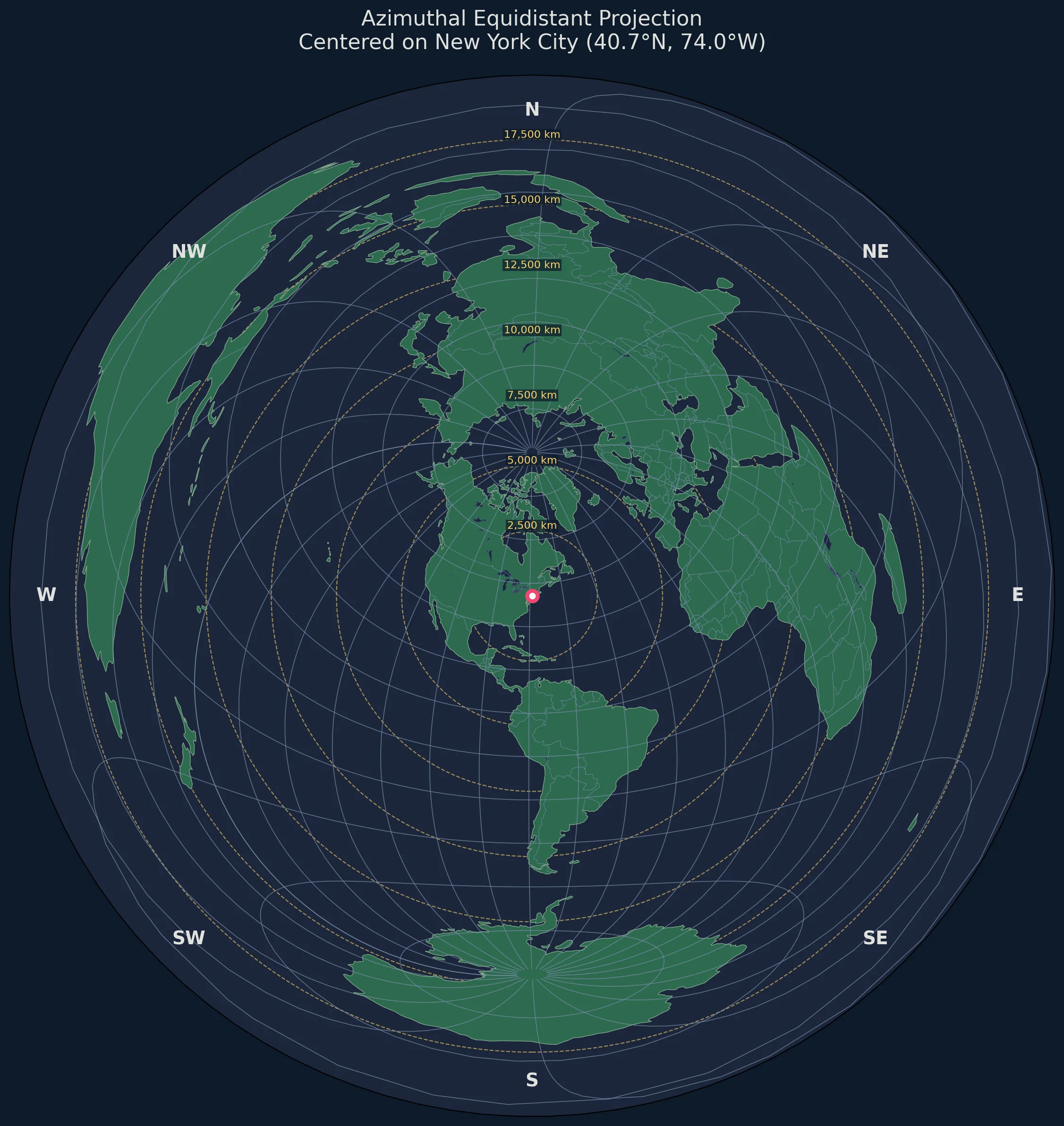
# Add title
plt.title(f'Azimuthal Equidistant Projection\nCentered on {center_lat}°N, {abs(center_lon)}°W',
fontsize=14, color='#e0e1dd', pad=20)
plt.tight_layout()
plt.savefig('azimuthal_map.png', dpi=150, bbox_inches='tight',
facecolor='#0d1b2a', edgecolor='none')
plt.show()
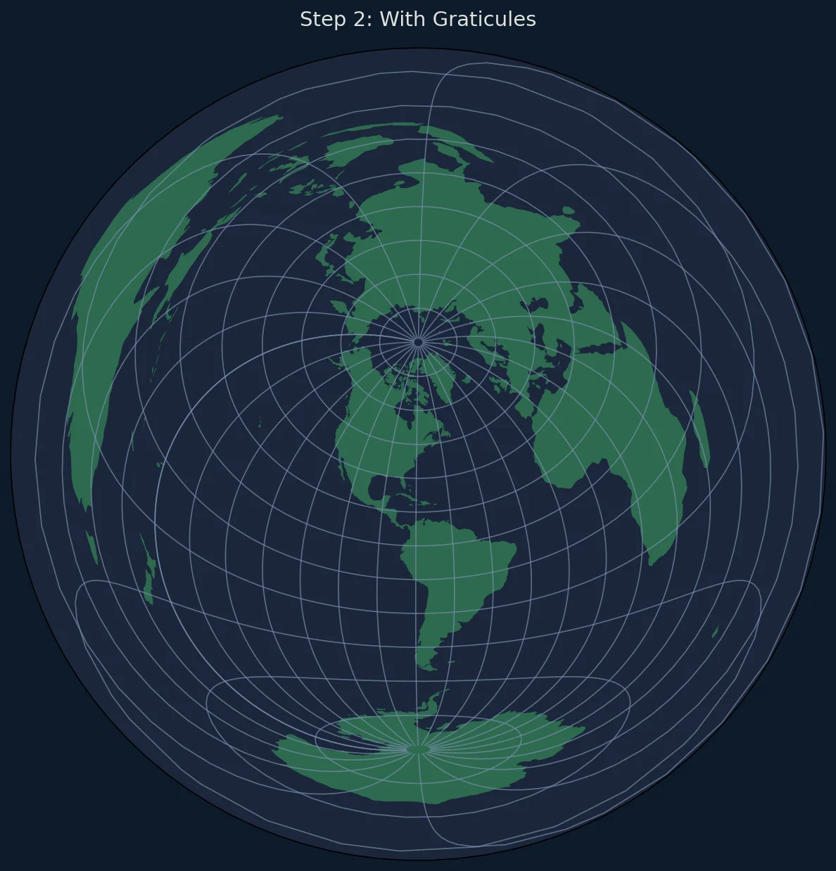
Adding Graticules (Grid Lines)
Graticules help readers understand latitude and longitude on the projected map:
import numpy as np

def add_graticules(ax, step=15):
    """Add latitude/longitude grid lines."""

    # Create gridlines with higher contrast
    gl = ax.gridlines(
        crs=ccrs.PlateCarree(),
        draw_labels=False,
        linewidth=0.6,
        color='#778da9',
        alpha=0.7,
        linestyle='-'
    )

    # Set grid spacing
    gl.xlocator = plt.FixedLocator(np.arange(-180, 181, step))
    gl.ylocator = plt.FixedLocator(np.arange(-90, 91, step))

    return gl

# Usage
add_graticules(ax, step=15)
Drawing Distance Rings
Distance rings are essential for azimuthal equidistant maps—they show true distances from the center:
import matplotlib.patches as mpatches
from matplotlib.collections import PatchCollection

def add_distance_rings(ax, center_lat, center_lon, distances_km, proj):
    """
    Add concentric distance rings around the center point.

    Parameters:
    -----------
    ax : matplotlib axes
    center_lat, center_lon : float
        Center point coordinates
    distances_km : list
        List of distances in kilometers for rings
    proj : cartopy projection
        The map projection
    """

    for distance in distances_km:
        # Convert km to meters (projection units)
        radius_m = distance * 1000

        # Create circle patch
        circle = plt.Circle(
            (0, 0),  # Center is at origin in projected coordinates
            radius_m,
            fill=False,
            edgecolor='#ffd166',
            linewidth=1,
            linestyle='--',
            alpha=0.7,
            transform=proj
        )
        ax.add_patch(circle)

        # Add distance label
        # Place label at top of ring (north direction)
        label_y = radius_m
        ax.text(
            0, label_y,
            f'{distance:,} km',
            fontsize=9,
            color='#ffd166',
            ha='center',
            va='bottom',
            transform=proj,
            bbox=dict(boxstyle='round,pad=0.2', facecolor='#0d1b2a',
                     edgecolor='none', alpha=0.7)
        )

# Usage
distances = [2500, 5000, 7500, 10000, 12500, 15000, 17500]
add_distance_rings(ax, center_lat, center_lon, distances, ax.projection)

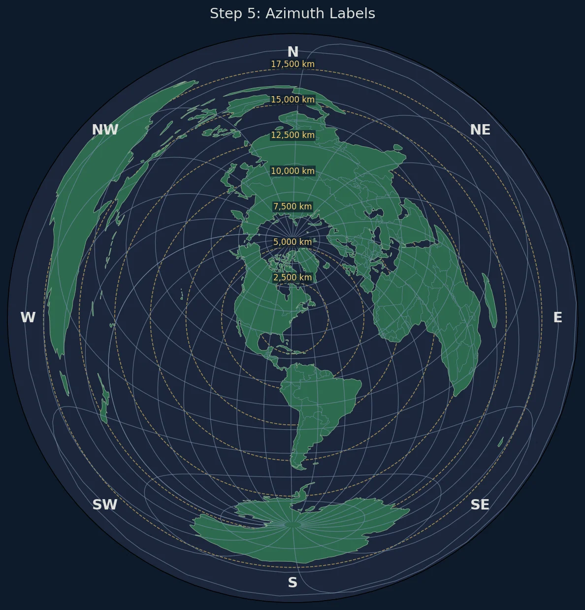
Adding Azimuth Labels
Compass directions around the map edge help with navigation:
def add_azimuth_labels(ax, radius_m):
    """Add compass direction labels around the map edge."""

    directions = [
        (0, 'N'), (45, 'NE'), (90, 'E'), (135, 'SE'),
        (180, 'S'), (225, 'SW'), (270, 'W'), (315, 'NW')
    ]

    for angle, label in directions:
        # Convert angle to radians (0° is North, clockwise)
        rad = np.radians(90 - angle)  # Adjust for math convention

        # Calculate position just inside the boundary
        label_radius = radius_m * 0.95
        x = label_radius * np.cos(rad)
        y = label_radius * np.sin(rad)

        ax.text(
            x, y, label,
            fontsize=12,
            fontweight='bold',
            color='#e0e1dd',
            ha='center',
            va='center',
            transform=ax.projection
        )

    # Add degree markers
    for angle in range(0, 360, 30):
        if angle % 45 != 0:  # Skip cardinal directions
            rad = np.radians(90 - angle)
            label_radius = radius_m * 0.92
            x = label_radius * np.cos(rad)
            y = label_radius * np.sin(rad)

            ax.text(
                x, y, f'{angle}°',
                fontsize=8,
                color='#778da9',
                ha='center',
                va='center',
                transform=ax.projection
            )

# Usage
add_azimuth_labels(ax, max_distance * 0.95)
Adding a Center Marker
Mark the projection center point:
def add_center_marker(ax, center_lat, center_lon, style='crosshair'):
    """
    Add a marker at the map center.

    Parameters:
    -----------
    style : str
        'dot', 'crosshair', or 'both'
    """
    from cartopy.crs import PlateCarree

    if style in ('dot', 'both'):
        ax.plot(
            center_lon, center_lat,
            'o',
            color='#ef476f',
            markersize=8,
            transform=PlateCarree(),
            zorder=10
        )

    if style in ('crosshair', 'both'):
        # Draw crosshair lines
        cross_size = 500000  # 500 km

        # Horizontal line
        ax.plot(
            [-cross_size, cross_size], [0, 0],
            color='#ef476f',
            linewidth=1.5,
            transform=ax.projection,
            zorder=9
        )

        # Vertical line
        ax.plot(
            [0, 0], [-cross_size, cross_size],
            color='#ef476f',
            linewidth=1.5,
            transform=ax.projection,
            zorder=9
        )

# Usage
add_center_marker(ax, center_lat, center_lon, style='both')
Plotting Custom Points
Add cities, stations, or other points of interest:
def plot_locations(ax, locations, center_lat, center_lon):
    """
    Plot multiple locations with distance annotations.

    Parameters:
    -----------
    locations : list of dict
        Each dict has 'name', 'lat', 'lon'
    """
    from cartopy.crs import PlateCarree, Geodetic
    from geopy.distance import geodesic

    for loc in locations:
        lat, lon = loc['lat'], loc['lon']
        name = loc['name']

        # Calculate true distance from center
        distance = geodesic(
            (center_lat, center_lon),
            (lat, lon)
        ).kilometers

        # Plot point
        ax.plot(
            lon, lat,
            'o',
            color='#06d6a0',
            markersize=6,
            transform=PlateCarree(),
            zorder=8
        )

        # Add label with distance
        ax.text(
            lon, lat,
            f' {name}\n {distance:,.0f} km',
            fontsize=8,
            color='#e0e1dd',
            transform=PlateCarree(),
            ha='left',
            va='top'
        )

# Example usage
cities = [
    {'name': 'London', 'lat': 51.5074, 'lon': -0.1278},
    {'name': 'Tokyo', 'lat': 35.6762, 'lon': 139.6503},
    {'name': 'Sydney', 'lat': -33.8688, 'lon': 151.2093},
    {'name': 'São Paulo', 'lat': -23.5505, 'lon': -46.6333},
    {'name': 'Moscow', 'lat': 55.7558, 'lon': 37.6173},
]

plot_locations(ax, cities, center_lat, center_lon)
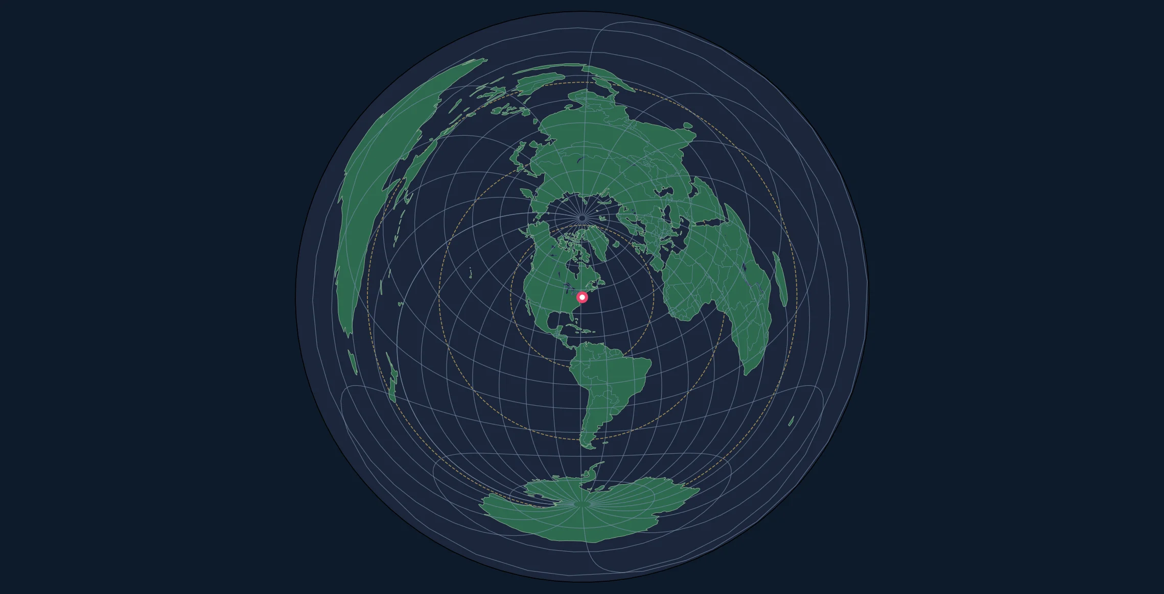
Complete Working Example
Here's a full script that combines all the elements:
#!/usr/bin/env python3
"""
Generate an azimuthal equidistant map centered on any location.
"""
import matplotlib.pyplot as plt
import matplotlib.patches as mpatches
import cartopy.crs as ccrs
import cartopy.feature as cfeature
import numpy as np
def create_azimuthal_map(center_lat, center_lon, title=None, filename=None):
"""
Create a complete azimuthal equidistant map.
Parameters:
-----------
center_lat : float
Latitude of center point
center_lon : float
Longitude of center point
title : str, optional
Map title
filename : str, optional
Output filename (saves if provided)
Returns:
--------
fig, ax : matplotlib figure and axes
"""
# Create projection
proj = ccrs.AzimuthalEquidistant(
central_longitude=center_lon,
central_latitude=center_lat
)
# Setup figure
fig = plt.figure(figsize=(12, 12), facecolor='#0d1b2a')
ax = fig.add_subplot(1, 1, 1, projection=proj)
# Set extent (full globe)
max_distance = 20000000 # 20,000 km
ax.set_extent(
[-max_distance, max_distance, -max_distance, max_distance],
crs=proj
)
# Background
ax.set_facecolor('#0d1b2a')
# Add map boundary circle
boundary = plt.Circle(
(0, 0), max_distance,
transform=proj,
fill=False,
edgecolor='#415a77',
linewidth=2
)
ax.add_patch(boundary)
# Add features
ax.add_feature(cfeature.OCEAN, facecolor='#1b263b', zorder=1)
ax.add_feature(cfeature.LAND, facecolor='#2d6a4f', edgecolor='none', zorder=2)
ax.add_feature(cfeature.COASTLINE, linewidth=0.5, edgecolor='#84a98c', zorder=3)
ax.add_feature(cfeature.BORDERS, linewidth=0.3, edgecolor='#778da9', zorder=3)
ax.add_feature(cfeature.LAKES, facecolor='#1b263b', edgecolor='#415a77',
linewidth=0.3, zorder=2)
# Graticules
gl = ax.gridlines(
crs=ccrs.PlateCarree(),
linewidth=0.3,
color='#415a77',
alpha=0.5,
linestyle='-'
)
gl.xlocator = plt.FixedLocator(np.arange(-180, 181, 15))
gl.ylocator = plt.FixedLocator(np.arange(-90, 91, 15))
# Distance rings
ring_distances = [2500, 5000, 7500, 10000, 12500, 15000, 17500]
for dist in ring_distances:
radius = dist * 1000
circle = plt.Circle(
(0, 0), radius,
transform=proj,
fill=False,
edgecolor='#ffd166',
linewidth=0.8,
linestyle='--',
alpha=0.6
)
ax.add_patch(circle)
# Label
ax.text(
0, radius, f'{dist:,} km',
fontsize=8, color='#ffd166',
ha='center', va='bottom',
transform=proj,
bbox=dict(facecolor='#0d1b2a', edgecolor='none',
alpha=0.7, pad=1)
)
# Azimuth labels
directions = [
(0, 'N'), (45, 'NE'), (90, 'E'), (135, 'SE'),
(180, 'S'), (225, 'SW'), (270, 'W'), (315, 'NW')
]
label_radius = max_distance * 0.93
for angle, label in directions:
rad = np.radians(90 - angle)
x = label_radius * np.cos(rad)
y = label_radius * np.sin(rad)
ax.text(x, y, label, fontsize=14, fontweight='bold',
color='#e0e1dd', ha='center', va='center', transform=proj)
# Center marker
ax.plot(0, 0, 'o', color='#ef476f', markersize=10,
transform=proj, zorder=10)
ax.plot(0, 0, 'o', color='#ef476f', markersize=6,
markerfacecolor='white', transform=proj, zorder=11)
# Title
if title is None:
title = f'Azimuthal Equidistant Projection\n{center_lat:.2f}°{"N" if center_lat >= 0 else "S"}, {abs(center_lon):.2f}°{"E" if center_lon >= 0 else "W"}'
ax.set_title(title, fontsize=16, color='#e0e1dd', pad=20)
ax.set_aspect('equal')
plt.tight_layout()
if filename:
plt.savefig(
filename,
dpi=200,
bbox_inches='tight',
facecolor='#0d1b2a',
edgecolor='none'
)
print(f"Map saved to {filename}")
return fig, ax
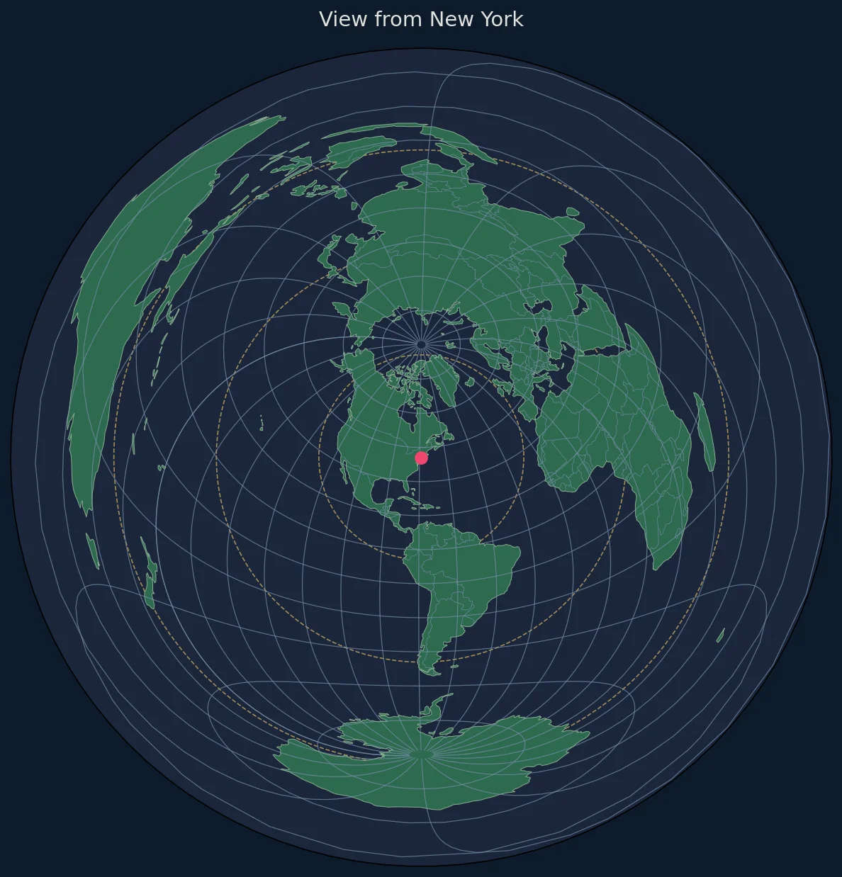
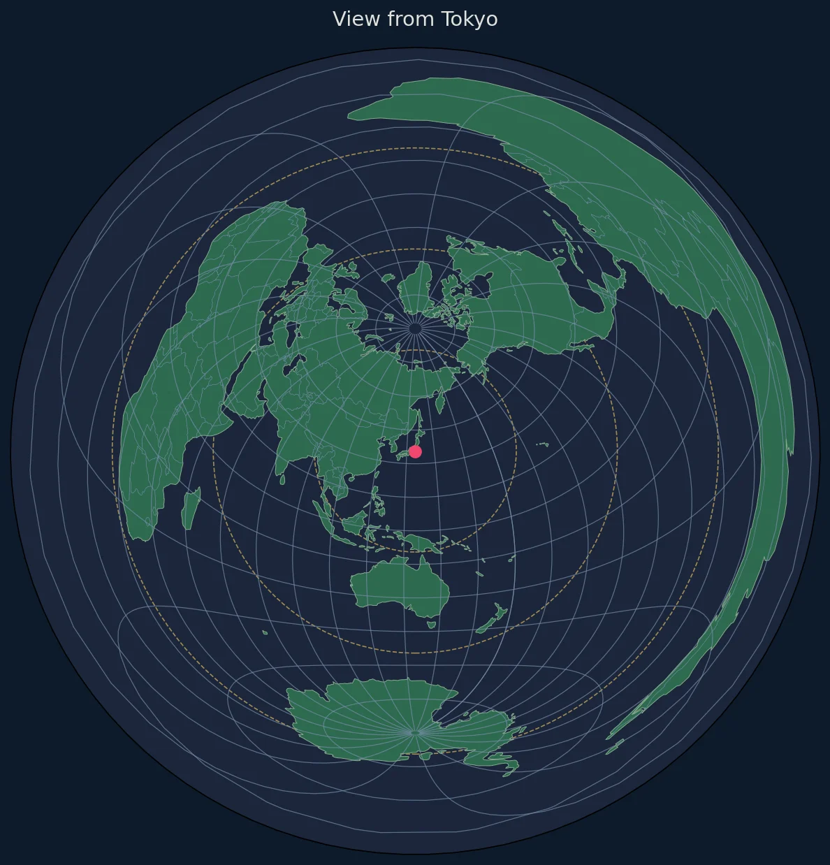
if __name__ == '__main__':
# Example: Create maps for several cities
locations = [
(40.7128, -74.0060, 'New York'),
(51.5074, -0.1278, 'London'),
(35.6762, 139.6503, 'Tokyo'),
(-33.8688, 151.2093, 'Sydney'),
]
for lat, lon, name in locations:
fig, ax = create_azimuthal_map(
lat, lon,
title=f'View from {name}',
filename=f'azimuthal_{name.lower().replace(" ", "_")}.png'
)
plt.close(fig)
print("All maps generated!")
Exporting High-Resolution Maps
For Print (300 DPI)
plt.savefig(
    'map_print.png',
    dpi=300,
    bbox_inches='tight',
    facecolor='white',  # White background for print
    edgecolor='none'
)
For Web (Optimized PNG)
plt.savefig(
    'map_web.png',
    dpi=150,
    bbox_inches='tight',
    facecolor='#0d1b2a',
    optimize=True
)

# Convert to WebP for better compression
# pip install pillow
from PIL import Image
img = Image.open('map_web.png')
img.save('map_web.webp', 'WEBP', quality=85)
Vector Format (SVG/PDF)
# SVG - ideal for web, scales infinitely
plt.savefig('map.svg', format='svg', bbox_inches='tight')

# PDF - ideal for print documents
plt.savefig('map.pdf', format='pdf', bbox_inches='tight')
Batch Processing Multiple Locations
Generate maps programmatically:
import pandas as pd

def batch_generate_maps(locations_csv, output_dir='maps/'):
    """
    Generate maps for a list of locations from CSV.

    CSV format: name,latitude,longitude
    """
    import os
    os.makedirs(output_dir, exist_ok=True)

    df = pd.read_csv(locations_csv)

    for _, row in df.iterrows():
        name = row['name']
        lat = row['latitude']
        lon = row['longitude']

        safe_name = name.lower().replace(' ', '_').replace(',', '')
        filename = f"{output_dir}/azimuthal_{safe_name}.png"

        fig, ax = create_azimuthal_map(lat, lon, title=f'View from {name}')
        plt.savefig(filename, dpi=150, bbox_inches='tight',
                   facecolor='#0d1b2a')
        plt.close(fig)

        print(f"Generated: {filename}")

# Usage
# batch_generate_maps('cities.csv')
Performance Considerations
For Large Datasets
# Use lower resolution coastlines for faster rendering
ax.add_feature(cfeature.COASTLINE.with_scale('110m'))  # Low res
ax.add_feature(cfeature.COASTLINE.with_scale('50m'))   # Medium res
ax.add_feature(cfeature.COASTLINE.with_scale('10m'))   # High res (slow)
Caching Projections
from functools import lru_cache

@lru_cache(maxsize=32)
def get_projection(center_lat, center_lon):
    """Cache projections for repeated use."""
    return ccrs.AzimuthalEquidistant(
        central_longitude=center_lon,
        central_latitude=center_lat
    )
Common Issues and Solutions
Issue: Map Appears Empty
# Solution: Check projection extent
ax.set_global()  # Or set specific extent in projection coordinates
Issue: Features Not Visible
# Solution: Check z-order
ax.add_feature(cfeature.LAND, zorder=1)  # Lower = drawn first
ax.add_feature(cfeature.BORDERS, zorder=2)  # Higher = on top
Issue: Slow Rendering
# Solution: Use lower resolution data
ax.add_feature(cfeature.NaturalEarthFeature(
    'physical', 'land', '110m',  # Use 110m instead of 10m
    facecolor='#2d6a4f'
))
Next Steps
- Create animated maps showing rotation
- Add custom shapefiles with GeoPandas
- Build an interactive version with D3.js
- Try the Lambert Equal-Area projection